DEMs (raster format) are created from point elevation observations. When working with a DEM, it is important to be aware that the values of a given cell are the result of some processing step that converted point elevations to a value at that location. Point data can be regularly (e.g. every 10 m along north and east directions) or irregularly spaced (i.e. all over the place). Different approaches are taken to convert these points to a DEM raster.

Unless you have all of the information regarding how a DEM was created (including estimates of uncertainty), you can only be truly confident in the values of a DEM if you do the point to raster conversion yourself. This is often glossed over.

This process can be carried out using various tools (python, gdal etc.) but I find the most succinct approach is to use the excellent libraries from R, namely raster and sp.

Note that there is a difference between interpolating a surface from points – interpolating values at locations where observations are not available – and creating a gridded representation of a point dataset. In the latter case, where data are not available, a grid cell will not have a value.

Regularly gridded points

Where you data are regularly gridded, you can take each point value and associate it directly with a grid cell.

R

R’s raster package provides functionality to create a raster from regularly gridded points rasterFromXYZ. To summarize the documentation:

NB/ If using the function and not specifying the raster resolution, it is assumed to be the minimum distance between x and y coordinates. Also, if the exact properties of the RasterLayer are known beforehand, it may be preferable to simply create a new RasterLayer with the raster function instead, compute cell numbers and assign the values with these.

Usage:

rasterFromXYZ(xyz, res=c(NA,NA), crs=NA, digits=5)

Example:

# create some regularly gridded point data:
library(raster)

r <- raster(nrow=10, ncol=10, xmn=0, xmx=10, ymn=0, ymx=10, crs=NA) # empty raster
r[] <- runif(ncell(r)) 												# set values of raster between 0 and 1 
r[r<0.5] <- NA 														# set some to NA
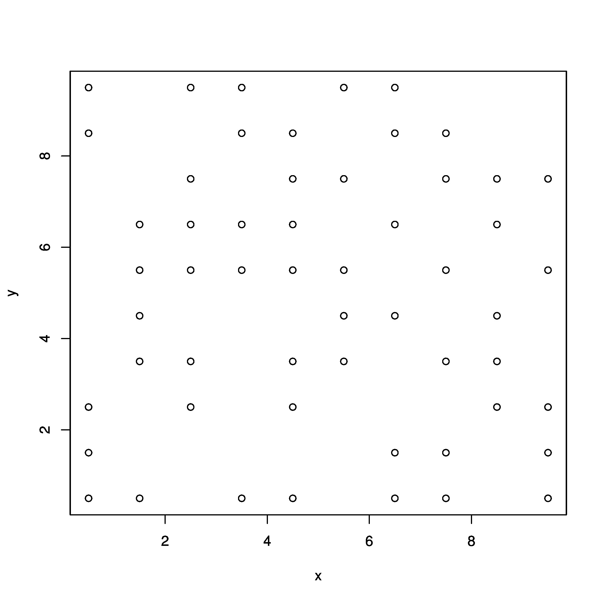
xyz <- rasterToPoints(r) 											# create regularly gridded points

Which look like:

# create raster from points
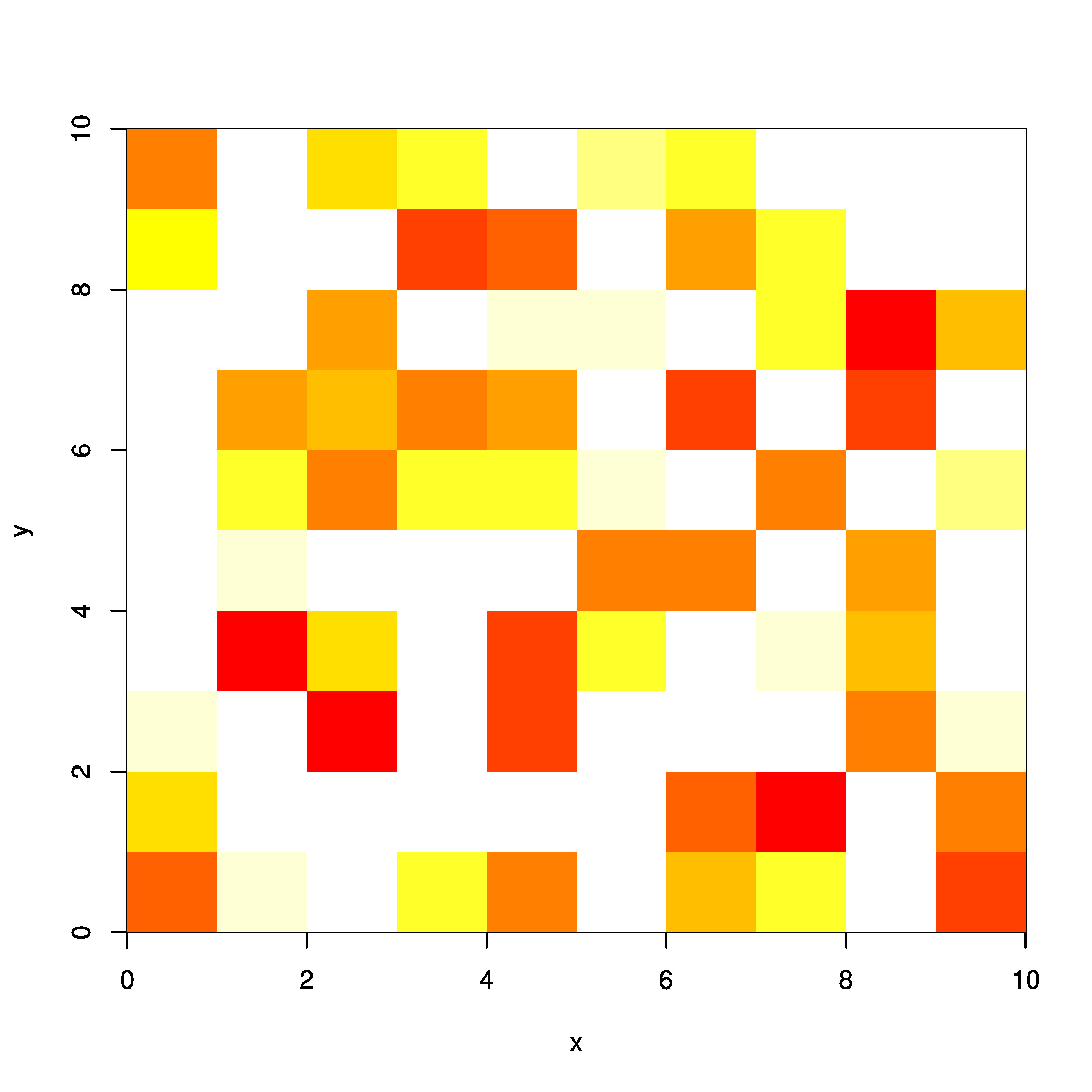
r2 <- rasterFromXYZ(xyz) 

Which gives:

Equally, you can compute the cell indices and assigning them with values:

r3 <- raster(nrow=10, ncol=10, xmn=0, xmx=10, ymn=0, ymx=10) 		# create empty raster
cells <- cellFromXY(r3, xyz[,1:2]) 									# compute cell numbers
r3[cells] <- xyz[,3] 												# assign values to cells

Look at the various cellFrom() functions in raster to see various ways to manipulate cell coordinates to grid positions.

Python

To do the equivalent in Python, we can make use of numpy. An excellent walk through of the process from Joe Kington is available here - a modified version of the link is presented below (partly in case the link breaks!)…

If your x and y values correspond to indices, you can do something similar to this:

import numpy as np

x = [0, 0, 1, 1, 2, 2]
y = [1, 2, 0, 1, 1, 2]
z = [14, 17, 15, 16, 18, 13]

z_array = np.nan * np.empty((3,3))
z_array[y, x] = z

print(z_array)

Which yields:

array([[ nan  15.  nan]
	  [ 14.  16.  18.]
	  [ 17.  nan  13.]])

If you have regularly sampled x & y points, then you can convert them to grid indices by subtracting the “corner” of your grid (i.e. x0 and y0), dividing by the cell spacing, and casting as ints. You can then use the method above. We can make an example assuming our top left coordinates are -800,-3400) (x,y) e.g.

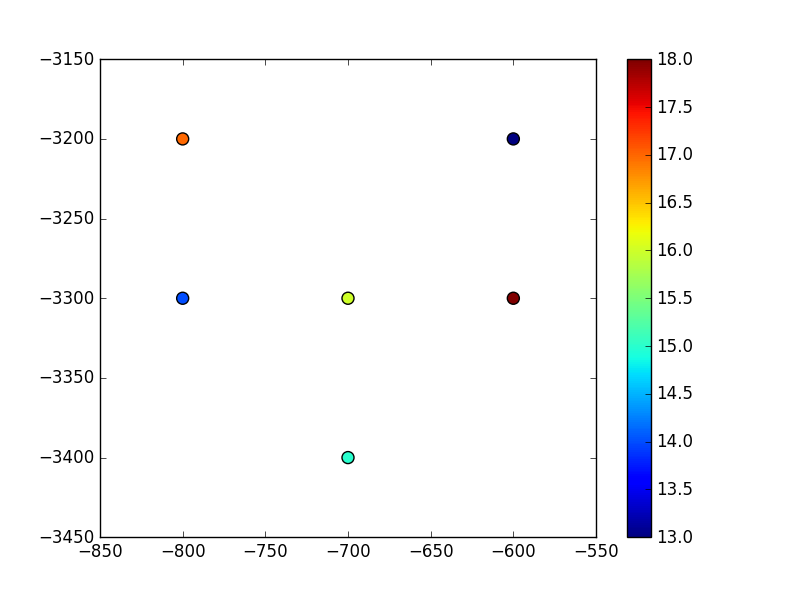
x = np.array([-800, -800, -700, -700, -600, -600])
y = np.array([-3300, -3200, -3400, -3300, -3300, -3200])
z = np.array([14, 17, 15, 16, 18, 13])

Our points look like:

Now we set the origin and convert the (x,y) coordinates to grid vertices:

x0=-800 	# x origin
y0=-3400 	# y origin
dy=100 		# y cell size
dx=100 		# x cell size

i = ((y - y0) / dy).astype(int) # y locations as grid indices
j = ((x - x0) / dx).astype(int) # x locations as grid indices

grid = np.nan * np.empty((len(y)/2,len(x)/2)) # numpy arrays read (y,x) not (x,y)!
grid[i,j] = z

Which yields:

array([[ nan,  15.,  nan],
      [ 14.,  16.,  18.],
      [ 17.,  nan,  13.]])

And looks like:

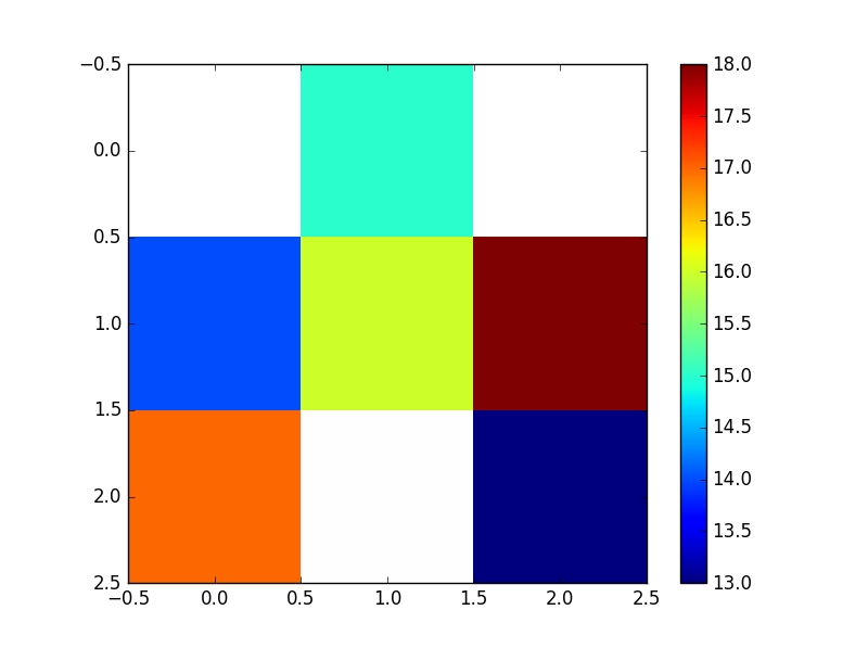
NB/ Remember that Python considers the grid origin to be the top left corner - if -800 (x) and -3400 (y) were actually the bottom left corner of the grid, you would want to flip the resultant grid i.e. grid[::-1]. This is why the values on the plot above are flipped compared to the earlier scatter of the input points. A flipped array looks like the below (the numpy indices have been left on though to illustrate numpy’s top left origin).

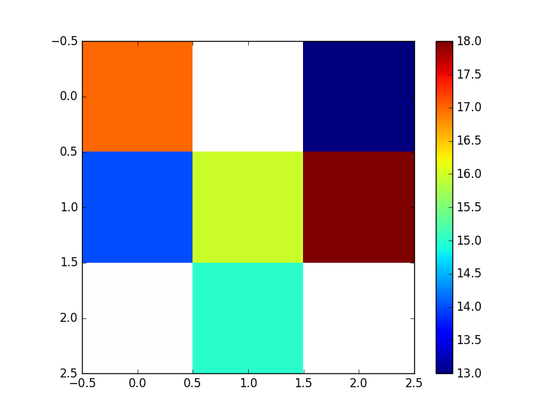
To output the numpy array to a raster (e.g. a geotiff), you need to make use of the gdal python bindings.

Irregularly gridded points

Often, your data won’t be regularly spaced. Now you need to consider methods specifically dealing with this, including the conversion of your points to regularly gridded data, which will require averaging or some sort of function. What if multiple points fall within the area of a raster cell?

R Code

Using R, irregular points can be converted to a grid using raster’s rasterize function.

library(raster)
library(sp)

f<-"/your/path/irregular_points.xyz"
pts <- read.table(f, header=FALSE, col.names=c("x", "y", "z")) # change accordingly - use read.csv for a csv!

# create a SpatialPointsDataFrame
coordinates(pts) = ~x+y 									   

# create an empty raster object to the extent of the points
rast <- raster(ext=extent(pts), resolution=250)

# rasterize your irregular points 
rasOut<-rasterize(pts, rast, pts$z, fun = mean) # we use a mean function here to regularly grid the irregular input points

#write it out as a geotiff
fout="my_raster.tif"
writeRaster(rasOut, fout, format="GTiff")

Python equivalent…

The equivalent in python can again be achieved using numpy a fantastic overview of the process again available here from Joe Kington. To summarize, irregular points can be binned onto a grid through use of numpy’s histogram function:

import numpy as np
import matplotlib.pyplot as plt

# Make some random data
np.random.seed(1977)
x, y, z = np.random.random((3, 50))

# Bin the data onto a 10x10 grid
# Have to reverse x & y due to row-first indexing
zi, yi, xi = np.histogram2d(y, x, bins=(10,10), weights=z, normed=False)
counts, _, _ = np.histogram2d(y, x, bins=(10,10))

zi = zi / counts
zi = np.ma.masked_invalid(zi)

#plot it
fig, ax = plt.subplots()
ax.pcolormesh(xi, yi, zi, edgecolors='black')
scat = ax.scatter(x, y, c=z, s=200)
fig.colorbar(scat)
ax.margins(0.05)

plt.show()

Which looks like this:

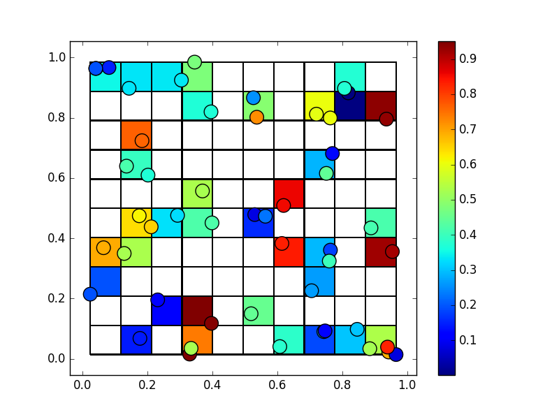
Again, to get this into a geotiff, have a look at the gdal python bindings.