Calculating the concave hull of a point data set (Python and R)

Following the calculation of a convex hull as described a few weeks ago, I’ve worked up a way to approximate a “concave” hull. This can be useful for point clouds of complicated geometries. Whereas the convex hull is a well defined concept, concave hulls are less so, verging on the subjective. That’s why I keep using “ “ around “concave hull”.

So, considering this potential subjectiveness, the method here actually calculates the hull from an applied kernel density function. The first thing to do is to calculate your kernel density function for a point cloud, which I’ve facilitated in R (albeit after reading this):

library(MASS)
library(scatterplot3d)
library(ggplot2)

# Read in and assign data
points <- read.csv("YOUR_file", sep=",", header=F)
xx <- points[[1]]
yy <- points[[2]]

# Calculate kernel density function
dens <- kde2d(xx, yy)
densdf <- data.frame(expand.grid(easting = dens$x, northing = dens$y), density = as.vector(dens$z))

write.table(densdf, "YOUR_output_table", sep="\t")

Python is then used to acquire contours from the density surface created above in R. This is all simplified from the main program to get to the point (I have integrated numerous checks through developing plots etc. The full program is available on github but the info below should suffice…) Firstly, you’ll need the following imports:

from scipy import ndimage
import matplotlib.pyplot as plt
import matplotlib.mlab as ml
import pandas as pd

Everything is then called by the following driver script:

def density_hull_approximator(density_xyz_file):
	
	## get x, y and density values from the R output into variables
	x,y,z = get_density_xyz(density_xyz_file)	
	
	## grid and log the density xyz data
	Z_log = grid_log_density(x,y,z) 

	## create smooth density surface and calculate plot extent
	smooth, extent = smooth_density_surface_points(Z_log, x, y) 
	
	## Create contour surface
	cs = grid_contour(smooth, extent, density_boundary)
	
	## Get contour vertices
	contour_x_list, contour_y_list = contour_vertices(cs)

This driver function calls the following functions. The first simply pulls in the density data created in R into variables:

def get_density_xyz(density_xyz_file):
	sep='\t'
	f = open(density_xyz_file, 'r')
	df = pd.read_csv(f, sep=sep, names=[ 'xx', 'yy', 'zz' ], header=0)
	x = df['xx']
	y = df['yy']
	z = df['zz']

	x = x.values
	y = y.values
	z = z.values
	return x, y, z

The x,y,z data is then gridded and logged:

def grid_log_density(x,y,z):
	xi = np.linspace(min(x), max(x))
	yi = np.linspace(min(y), max(y))
	X, Y = np.meshgrid(xi, yi)
	z_log = np.log(z)
	Z_log = ml.griddata(x, y, z_log, xi, yi)
	
	return Z_log

The logged density grid is then smoothed using a gaussian filter and the extent of the grid is acquired:

def smooth_density_surface_points(Z_log, x, y, density_to_nan_limit=-40):
	smooth = ndimage.filters.gaussian_filter(Z_log, sigma=1.0, order=0, mode='reflect')
	smooth[smooth<=density_to_nan_limit] = np.nan
	extent = (x.min(), x.max(), y.min(), y.max())

	return smooth, extent

The smoothed density grid is then contoured - the “level” variable is user set and must be specific to YOUR data and YOUR area/density contour of interest. It would be wise to actually view this plot and maybe cycle a number of density contour levels to know exactly what hull you are mapping:

	
def grid_contour(surface, extent, density_boundary):
	cs = plt.contour(surface, levels=[density_boundary], linewidth = 5, extent=extent)

	return cs

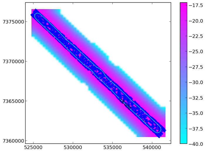
Such a plot could look like this:

"Concave hull" boundary - ideal

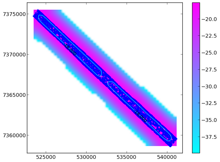
Equally, you WOULDN’T want it to look like this:

"Concave hull" boundary - not ideal

Now you have a contour that you have hopefully checked! The next thing to do is to get the vertices of the contour line - these form the xy coordinates of your “concave” mask:

	
def contour_vertices(cs):
	p = cs.collections[0].get_paths()[0]
	v = p.vertices
	contour_x = v[:,0]
	contour_y = v[:,1]
	contour_x_list = contour_x.tolist()
	contour_y_list = contour_y.tolist()

	return contour_x_list, contour_y_list

You can now save and export these lists. You now have the coordinates of your concave hull boundary.

Written on December 12, 2014